Have you ever wanted to find an image among your never-ending image dataset, but found it too tedious? In this tutorial we’ ll build an image similarity search engine to easily find images using either a text query or a reference image.
The semantic meaning of an image can be represented by a numerical vector called an embedding. Comparing these low-dimensional embedding vectors, rather than the raw images, allows for efficient similarity searches. For each image in the dataset, we’ ll create an embedding vector and store it in an index. When a text query or a reference image is provided, its embedding is generated and compared against the indexed embeddings to retrieve the most similar images.
Here’ s a brief overview:
The CLIP (Contrastive Language-Image Pre-training) model, developed by OpenAI, is a multi-modal vision and language model that maps images and text to the same latent space.Since we will use both image and text queries to search for images, we will use the CLIP model to embed our data.
FAISS (Facebook AI Similarity Search) is an open-source library developed by Meta. It is built around the Index object that stores the database embedding vectors. FAISS enables efficient similarity search and clustering of dense vectors, and we will use it to index our dataset and retrieve the photos that resemble to the query.
To create the image dataset for this tutorial I collected 52 images of varied topics from Pexels. To get the feeling, lets observe 10 random images:

To extract CLIP embeddings, we‘ ll first load the CLIP model using the HuggingFace SentenceTransformer library:
model=SentenceTransformer('clip-ViT-B-32')Next,
we’
ll create a function that iterates through our dataset directory with glob,
opens each image with PIL Image.open,
and generates an embedding vector for each image with CLIP model.encode. It returns a list of the embedding vectors and a list of the paths of our images dataset:
def generate_clip_embeddings(images_path, model):

image_paths=glob(os.path.join(images_path, '**/*.jpg'), recursive=True)

embeddings=[]
for img_path in image_paths:
image=Image.open(img_path)
embedding=model.encode(image)
embeddings.append(embedding)

return embeddings,
image_paths


IMAGES_PATH='/path/to/images/dataset'

embeddings,
image_paths=generate_clip_embeddings(IMAGES_PATH, model)
The next step is to create a FAISS index from the embedding vectors list. FAISS offers various distance metrics for similarity search, including Inner Product (IP) and L2 (Euclidean) distance.
FAISS also offers various indexing options. It can use approximation or compression technique to handle large datasets efficiently while balancing search speed and accuracy. In this tutorial we will use a ‘ Flat’ index, which performs a brute-force search by comparing the query vector against every single vector in the dataset, ensuring exact results at the cost of higher computational complexity.
def create_faiss_index(embeddings, image_paths, output_path):

dimension=len(embeddings[0])
index=faiss.IndexFlatIP(dimension)
index=faiss.IndexIDMap(index)

vectors=np.array(embeddings).astype(np.float32)

# Add vectors to the index with IDs
index.add_with_ids(vectors, np.array(range(len(embeddings))))

# Save the index
faiss.write_index(index, output_path)
print(f"Index created and saved to {output_path}")

# Save image paths
with open(output_path + '.paths', 'w') as f:
for img_path in image_paths:
f.write(img_path + '\n')

return index


OUTPUT_INDEX_PATH="/content/vector.index"
index=create_faiss_index(embeddings, image_paths, OUTPUT_INDEX_PATH)
The faiss.IndexFlatIPinitializes an Index for Inner Product similarity,
wrapped in an faiss.IndexIDMapto associate each vector with an ID. Next,
the index.add_with_idsadds the vectors to the index with sequential ID’
s,
and the index is saved to disk along with the image paths.
The index can be used immediately or saved to disk for future use .To load the FAISS index we will use this function:
def load_faiss_index(index_path):
index=faiss.read_index(index_path)
with open(index_path + '.paths', 'r') as f:
image_paths=[line.strip() for line in f]
print(f"Index loaded from {index_path}")
return index,
image_paths

index,
image_paths=load_faiss_index(OUTPUT_INDEX_PATH)
With our FAISS index built,
we can now retrieve images using either text queries or reference images. If the query is an image path,
the query is opened with PIL Image.open. Next,
the query embedding vector is extracted with CLIP model.encode.
def retrieve_similar_images(query, model, index, image_paths, top_k=3):

# query preprocess:
if query.endswith(('.png', '.jpg', '.jpeg', '.tiff', '.bmp', '.gif')):
query=Image.open(query)

query_features=model.encode(query)
query_features=query_features.astype(np.float32).reshape(1, -1)

distances,
indices=index.search(query_features, top_k)

retrieved_images=[image_paths[int(idx)] for idx in indices[0]]

return query,
retrieved_images
The Retrieval is happening on the index.searchmethod. It implements a k-Nearest Neighbors (kNN) search to find the kmost similar vectors to the query vector. We can adjust the value of k by changing the top_kparameter. The distance metric used in the kNN search in our implementation is the cosine similarity. The function returns the query and a list of retrieve images paths.
Search with a Text Query:
Now we are ready to examine the search results. The helper function visualize_resultsdisplays the results. You can fined it in the associated Colab notebook. Lets explore the retrieved most similar 3 images for the text query “
ball”
for example:
query='ball'
query,
retrieved_images=retrieve_similar_images(query, model, index, image_paths, top_k=3)
visualize_results(query, retrieved_images)

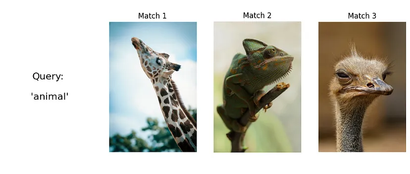
For the query ‘ animal’ we get:

Search with a Reference Image:
query='/content/drive/MyDrive/Colab Notebooks/my_medium_projects/Image_similarity_search/image_dataset/pexels-w-w-299285-889839.jpg'
query,
retrieved_images=retrieve_similar_images(query, model, index, image_paths, top_k=3)
visualize_results(query, retrieved_images)

As we can see, we get pretty cool results for an off-the-shelf pre-trained model. When we searched by a reference image of an eye painting, besides finding the original image, it found one match of eyeglass and one of a different painting. This demonstrates different aspects of the semantic meaning of the query image.